
Measurements of particle size distributions provide a large amount of data that can potentially reveal much about how particles are formed and processed in the atmosphere. Below is an example of the data that can be obtained. The figure shows one day's data measured with a DMA/CPC during the Pacific 2001  study at a site near Abbottsford, British Columbia. The figure consists of 8640 data points: 30 size bins (logarithmically spaced from 9 nm to 640 nm) measured at 288 times (every 5 minutes). The color scale gives the number of particles per cubic centimeter of air for each of these points.
There is a lot happening here. Most dramatic is the nucleation and growth event; this begins at about noon with the formation of a large number (shown in red) of very small particles that rapidly grow to diameters of several 10's of nanometers. But there are also a number of other smaller changes in the distributions.
Measurements like these potentially provide a great deal of information on how particles behave in the atmosphere. But one of the challenges with using this data is that there is so much of it - a typical field study, lasting several weeks, will produce several hundred thousand data points. That is really too much for the human brain to process without some form of simplification.
We have developed the application of a statistical technique called principal component analysis as a tool in simplifying and interpreting these complex data sets. This work was carried out by Tak Chan, a graduate student in the Mozurkewich group who completed his PhD in 2005. The basic idea is to factor a matrix of data into two smaller matrices, called "scores" and "loadings". For example, the size distribution data set described above would be put in the form of a matrix with 30 columns (one for each size bin) and some hundreds or thousands of rows (one for each measurement time). The size bins are then replaced by a smaller number of components, each of which has a certain size distribution; an example of these component loadings is shown on the right. Each component covers a fairly narrow range of sizes.
At each measurement time, there is a "score" for each component; these specify how much of the component is present at that time. Multiplying all the loadings by their respective scores and adding up the results regenerates the measured size distribution.
 Component loadings for an eight component fit to the Pacific 2001 data set. The size distribution for each component is shown in a different color. The curves are labeled with the diameters, in nm, at their maxima.
Representing Data with Components
With even a small number of components, virtually all the information in the measured distributions can be preserved. Below is an example of the fit for a portion of the Pacific 2001 study. The fit is to the data set for the entire study and is actually rather poor for the week shown. Even so, one must look rather closely to spot the areas where the fit differs greatly from the data. With eight components, the fit is virtually indistinguishable from the measured data. Since we have now replaced 30 variables with 5 to 8 variables, we have made the data much easier to interpret. (Software attached "Representing Data with Components")
 Top: One week's measured data. Bottom: Fitted data using five components.
Identifying Sources
 A common use of principal component analysis in atmospheric chemistry is the identification of sources. The analysis shown above does not do this; but it is a big help in source identification. Once we have simplified the size distribution data set, we can combine the scores with other measured variables, such as trace gas concentrations and meteorological data and then apply a second round of principal component analysis to this mixed data set. We have done this for data collected during four field campaigns in southern Ontario. Data were collected during the summers of 1999 and 2000 at a heavily polluted urban site in downtown Hamilton; during the summer of 2000 at Simcoe, a rural site that is heavily impacted by trans- boundary pollution from the U.S. midwest; and in the spring of 2003 at Egbert, a rural site that, depending on wind direction, received fresh pollutants from Toronto, clean air from the north and east, and aged polluted air from the U.S. midwest. The analysis shows some "factors" (a group of associated quantities) that are common to all sites and some that are specific to certain sites.
Regional Pollution Factor
The graph on the left shows the amounts of various measured quantities associated with this factor;  it consists mostly of accumulation mode particles (> 100 nm diameter), CO, and NOx. These are all associated with regional scale pollution. Similar results were obtained from the other data sets. For simultaneous measurements at Hamilton and Simcoe, the scores (amount of the factor present) were very similar; this is expected for regional scale pollution. The graphs below show the scores at Hamilton and Egbert. When the later site received polluted air from the south and southwest, the scores were similar to the scores at Hamilton. But the scores at Egbert were much smaller when the site received clean air from the forested areas to the north and east.

 Photochemical Nucleation Factor
This was observed at all the sites. As shown in the graph at right, it consists of extremely small particles (below 25 nm diameter) and has a strong association with the intensity of sunlight. The amount of this factor present always has a sharp peaks in late morning or near mid-day, this may be seen in the graph below. It is often thought that nucleation can not occur in the presence of a large aerosol surface area, but the graph below contradicts that since the urban Hamilton site had very high concentrations of particles even before nucleation occurred.
 Aitkin Particles
Aitken particles are intermediate in size between the nucleation and accumulation modes. They are present at all the sites, but with differing sources. The graph below on the left shows that at Egbert these particles have diameters of 30 to 100 nm and are associated with SO2. The graph below on the right shows the dependence of the scores on wind direction; the largest amounts are present when the wind is from the south, that is, from Toronto. Thus, it appears that this component consists of relatively fresh emissions, very likely from traffic.
 Aitken Particles in Hamilton
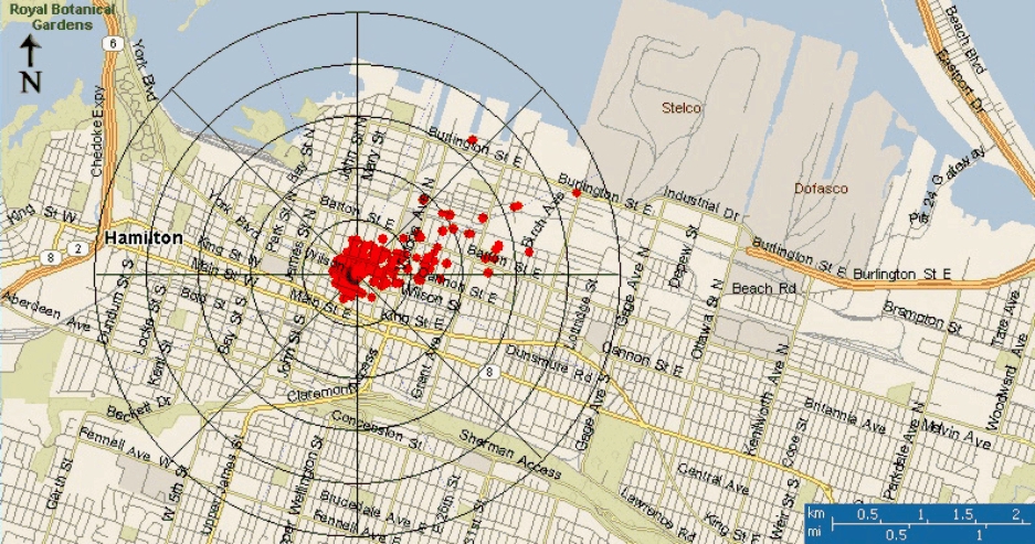
The graph on the right shows that, ss in Egbert, the Aitken particles in Hamilton have diameters of 30 to 100 nm and are associated with SO2. Very high scores are associated with one particular wind direction. Below, a plot of the scores versus wind direction is super-imposed on a map of Hamilton. The center of the plot is at the measurement site. The source appears to be the steel mills in Hamilton. 
Aitken Particles at Simcoe
 At Simcoe, the Aitken particles have a very different source. They are not emitted locally; instead, they are produced by growth following nucleation events. The graph on the right show that peaks in the nucleation component are followed by peaks in the Aitken component (labeled "growth" on the graph) as the newly formed particles grow into the larger size range.
Summary: Principal component analysis can be successfully applied to aerosol size distribution data, provided that suitable weighting is applied to the data. The effect is to replace a large number of size bins with only a few variables while preserving virtually all the information in the data. The resulting components can be used as inputs, along with trace gas and meteorological data, in a more conventional principal component analysis. This permits a degree of source identification.
Acknowledgments: Richard Leaitch and Jason O'Brien of the Meteorological Service of Canada provided the meteorological data used in these analyses. This work was supported by grants from the Canadian Foundation for Climate and Atmospheric Science and the Natural Science and Engineering Research Council of Canada.